Documentation
Delphy.ai
Welcome to Delphy.ai! This guide will walk you through the process of getting started with our app and help you quickly become familiar with its key features. By following these steps, you'll be up and running in no time.
- Version: 1.1
- Author: Dave Buell
- Created: 30 April, 2023
- Update: 10 May, 2023
If you have any questions that are beyond the scope of this help file, Please feel free to email via Item Support Page.
Account Creation
To begin using Delphy, you need to create an account. Follow the steps below to create your account and start experiencing the benefits of our app:
- Visit our website: Go to https://www.delphy.ai/ using any web browser.
- Sign Up: Look for the "Sign Up" button on the homepage or navigation menu and click on it.
- Provide your information: Fill in the required information in the sign-up form.
- Agree to Terms and Conditions: Read and accept the terms and conditions or user agreement for using Delphy.ai. Make sure you understand the terms before proceeding.
- Verify your email: After completing the sign-up form, you will receive a confirmation email at the email address you provided. Open the email and click on the verification link or follow the instructions to verify your email address. If you don't receive the email, check your spam or junk folder.
- Log in: Return to Delphy website and click on the "Sign In" button. Enter your registered username and password to access your account.
- Set up your profile (optional): Once your email is verified, you may have the option to set up your profile. This could include adding a profile picture, setting your preferences, or customizing your account settings. Take some time to personalize your profile to make the most of your experience.
Key Features
Delphy offers a comprehensive set of features designed specifically for algo traders looking to incorporate machine learning into their trading strategies. Let's explore the key features that make Delphy an essential tool for algorithmic trading.
Exploratory Data Analysis (EDA)
With Delphy's powerful EDA capabilities, you can analyze historical market data to gain valuable insights. Discover patterns, trends, and anomalies in the data to inform your trading strategies. Identify relevant features and refine your understanding of the underlying market dynamics.
Correlation Analysis
Efficiently evaluate the relationships between various technical indicators (features) and the target variable (price prediction). Delphy provides advanced correlation analysis tools that help you identify meaningful connections between different indicators and their impact on price movements. Leverage this knowledge to enhance the accuracy and performance of your trading models.
Machine Learning Strategy Creation
Delphy empowers you to create sophisticated machine learning-based trading strategies with ease. Utilize a range of machine learning algorithms and techniques, to build robust and adaptive trading models. Customize your strategies based on your preferred risk tolerance, time horizons, and other trading parameters.
Strategy Portfolio Management
Effortlessly organize and manage your machine learning strategies with Delphy's intuitive portfolio management system. Create and save multiple strategies within your portfolio, each tailored to different market conditions or asset classes. The portfolio view provides a consolidated overview of your strategies, allowing you to monitor their performance and make informed decisions.
Predictive Insights
Leverage your machine learning strategies to generate accurate and actionable predictions. Delphy seamlessly integrates your trained models with real-time market data, enabling you to make informed trading decisions based on predictive insights. Monitor market conditions, receive alerts, and execute trades directly from the platform, all while leveraging the power of machine learning.
EDA
EDA, or Exploratory Data Analysis, is a crucial step in the machine learning process. It involves the systematic examination of datasets to better understand their structure, identify patterns, anomalies, relationships between variables, and potential issues that may affect model performance.
Symbol Selection
To start an EDA, the following parameters must be specified:
Instrument
Choose the financial instrument you want to analyze from:
- Stocks
- ETFs
- Cryptocurrencies
- Forex
- Indices
For example, if you want to analyze the stock of Apple, you can select the instrument "Stocks".
Symbol
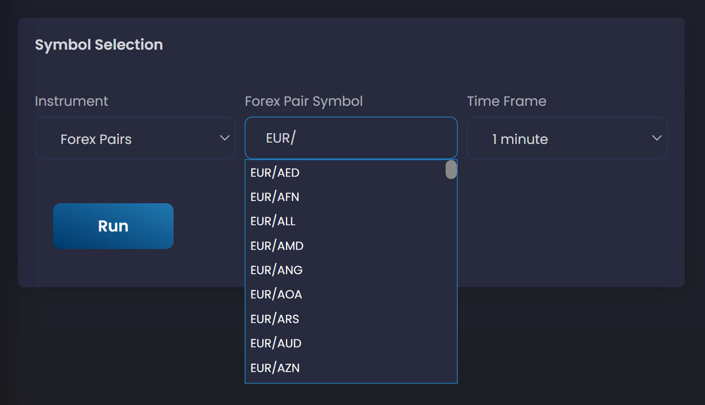
Once the instrument is selected, you can indicate the symbol by typing it into the input field. By typing at least two letters, Delphy will suggest all symbols that begin with those letters.
Time Frame
Finally, you can choose the time frame of the data you want to analyze. The time frame is the period during which data is considered for generating a single, aggregated data point.
The available time frames are:
- 1 minute
- 5 minutes
- 15 minutes
- 30 minutes
- 1 hour
- 4 hours
- 1 day
By choosing the time frame, you are setting the granularity of the financial data you are going to analyze.
Symbol Profile
Table where the main information related to the selected instrument is displayed.
Information displayed
If a Stock or ETF has been selected as instrument, a profile will be displayed with the following information:
- Name
- Exchange
- Country
- Sector
- Industry
- Type
- Description
Plots
Delphy provides two types of graphs to display data: Time Series chart and Histogram.
Time Series
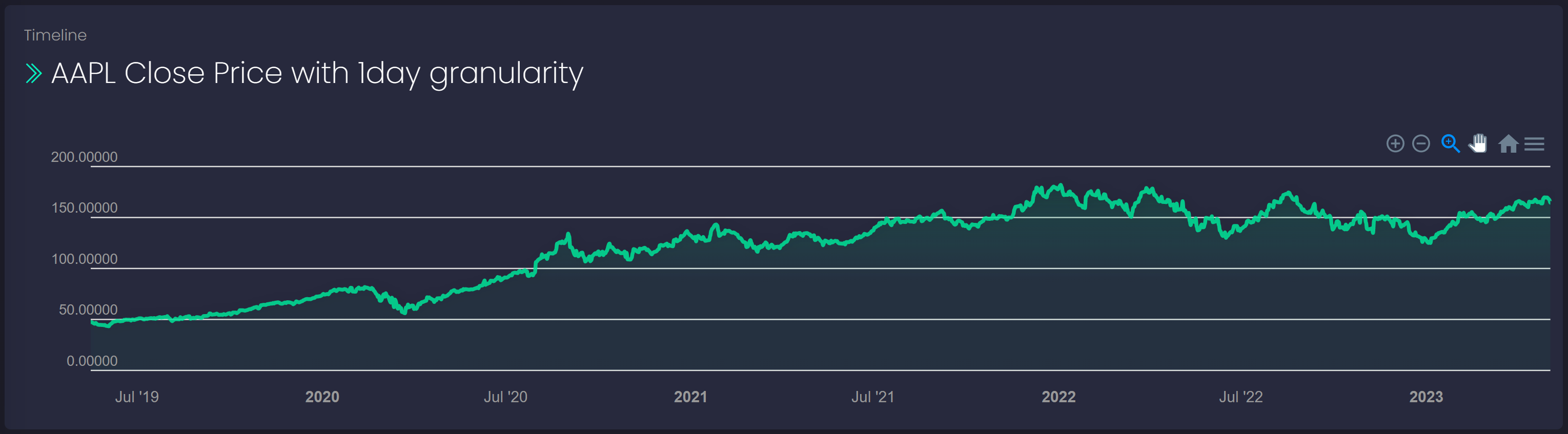
The Time Series chart shows the raw data of the symbol with the granularity selected in the time frame. For now, the viewable data range starts from the last available data point and goes back 2.000 points. The user can check the graph with the controls in the upper right and can download the data.
Histogram
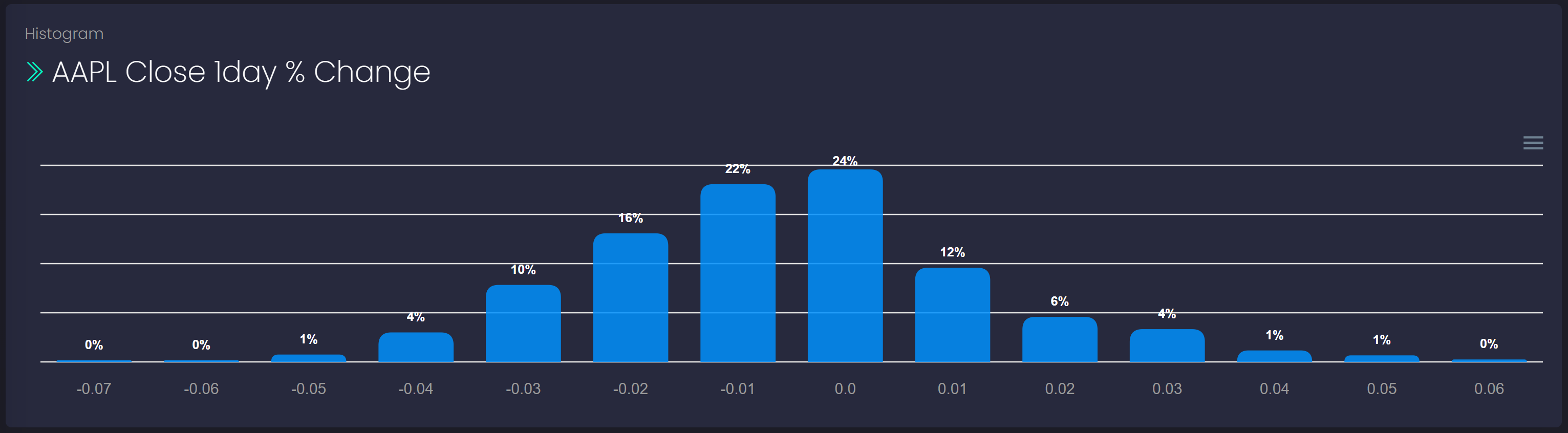
An histogram allows to understand the data's distributions. If it's a normal distribution, things like parametric statistics can be used.
On the X-axis there are the percentage changes in the instrument, while above each box it's shown the frequency in which that change occurs.
Data Table
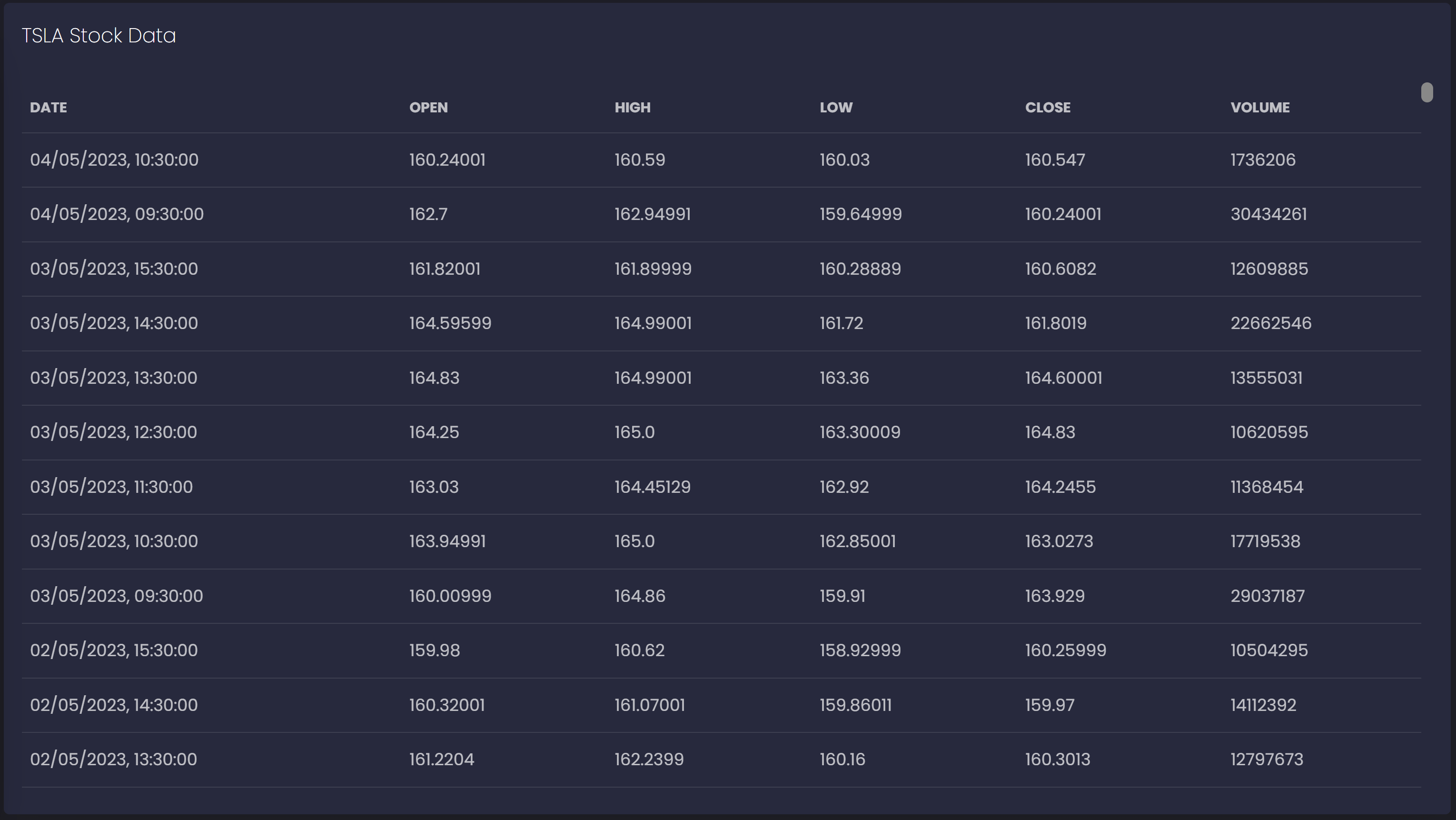
In the table below the graphs, all data points (OHLCV) of the selected instrument are shown with the chosen granularity.
Correlations
Correlations are nice to check out before building machine learning models, because we can see which features correlate to the target most strongly. Pearson's correlation coefficient is often used, which only detects linear relationships. It's commonly assumed our data is normally distributed, which we can "eyeball" from histograms. Highly correlated variables have a Pearson correlation coefficient near 1 (positively correlated) or -1 (negatively correlated). A value near 0 means the two variables are not linearly correlated.
Target Selection
To calculate correlations, we must first define our target. We want to predict the price trend of a financial instrument, so we are going to select the symbol as in the EDA section, but in addition we need the information of how far into the future we want to make the prediction.
Instrument
Choose the financial instrument you want to analyze from:
- Stocks
- ETFs
- Cryptocurrencies
- Forex
- Indices
For example, if you want to analyze the stock of Apple, you can select the instrument "Stocks".
Symbol
Once the instrument is selected, you can indicate the symbol by typing it into the input field. By typing at least two characters, Delphy will suggest all symbols that begin with those.
Time Frame
After that, you can choose the time frame of the data you want to analyze. The time frame is the period during which data is considered for generating a single, aggregated data point.
The available time frames are:
- 1 minute
- 5 minutes
- 15 minutes
- 30 minutes
- 1 hour
- 4 hours
- 1 day
By choosing the time frame, you are setting the granularity of the financial data you are going to analyze.
How far?
Finally, you can choose how far into the future you want to make the prediction. The available options are:
- 1 Days
- 2 Days
- 5 Days
- 15 Days
- 30 Days
Features Selection
For feature selection, 4 different indicators can be chosen. See the section Technical Indicators for more information about the indicators.
Heatmap
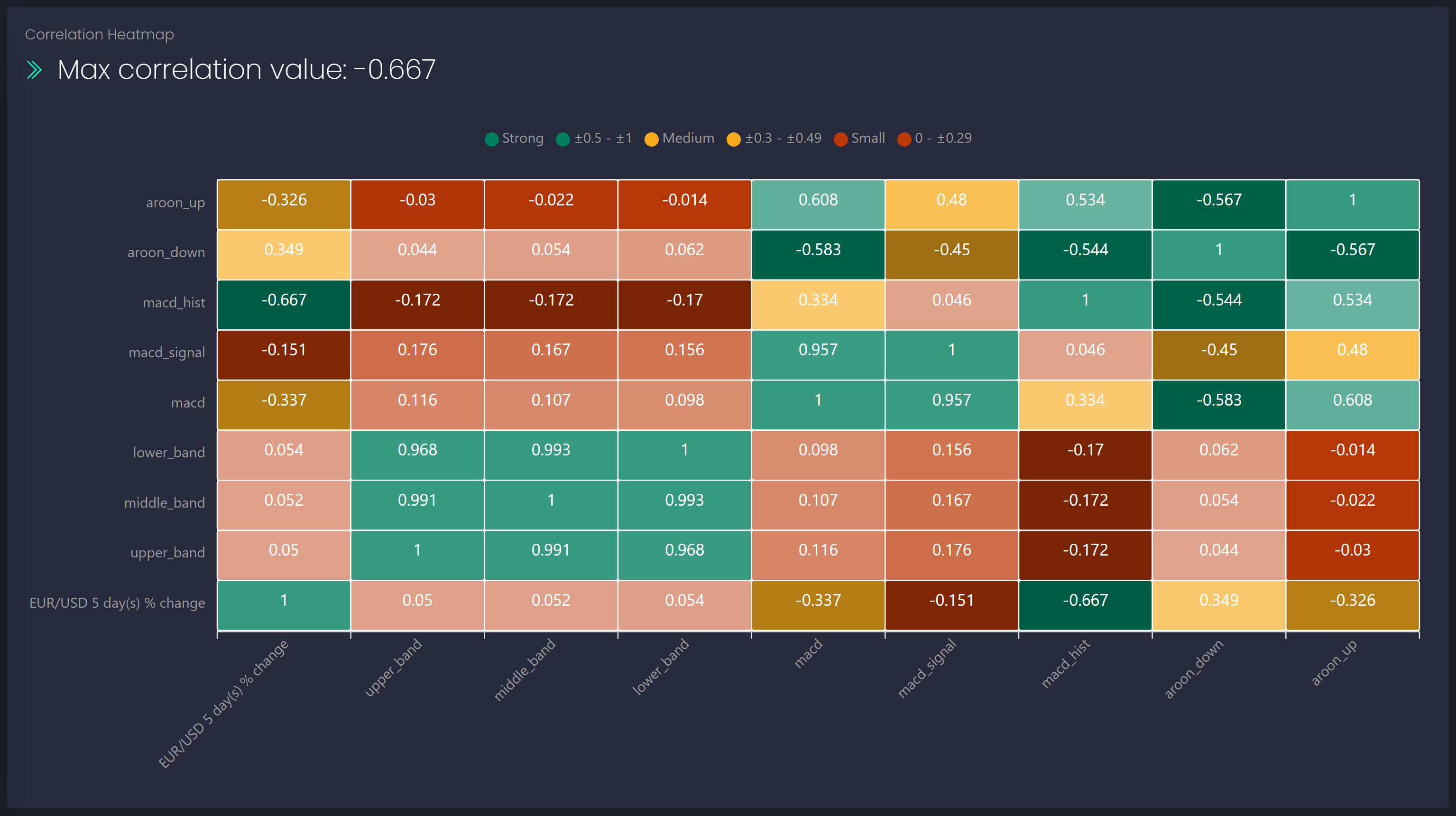
A correlation heatmap is a visual representation of the correlation matrix, which shows the pairwise relationships between variables in a dataset. It uses color gradients to depict the strength and direction of correlations, making it easy to identify patterns and potential associations among variables.
In our case, the most important row to examine is the bottom one, as it shows how well the indicators correlate with our target. If a technical indicator has multiple components, all will be examined in the correlation calculation and shown. For example, Bollinger Bands will have three components: upper_band, lower_band, and middle_band.
Scatter Plot
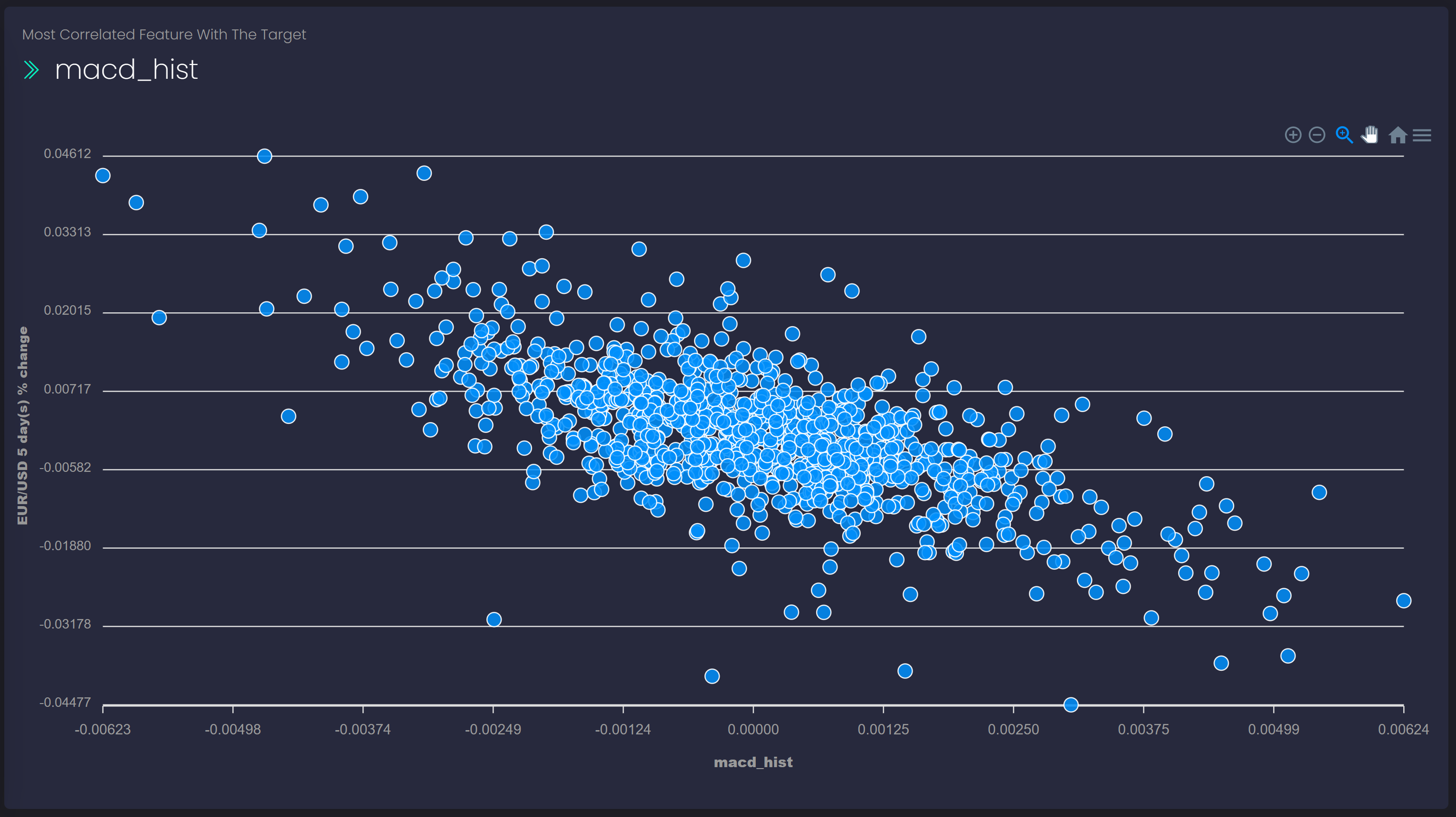
The Scatter Plot shows which feature correlates best with the target.
The Y-axis shows the target, i.e., the percentage change values of the chosen instrument. The X axis represents the feature that correlates best.
Machine Learning Strategies
Delphy aims to empower algotraders by providing the ability to leverage Machine Learning models for enhancing their trading strategies. In the next sections, we will discuss how Delphy allows users to build, test, and validate ML models, create tailored trading strategies, and perform backtesting for evaluating performance. Additionally, we will explore how Delphy enables users to save these strategies for daily usage.
What does it mean to create and use a strategy with Delphy?
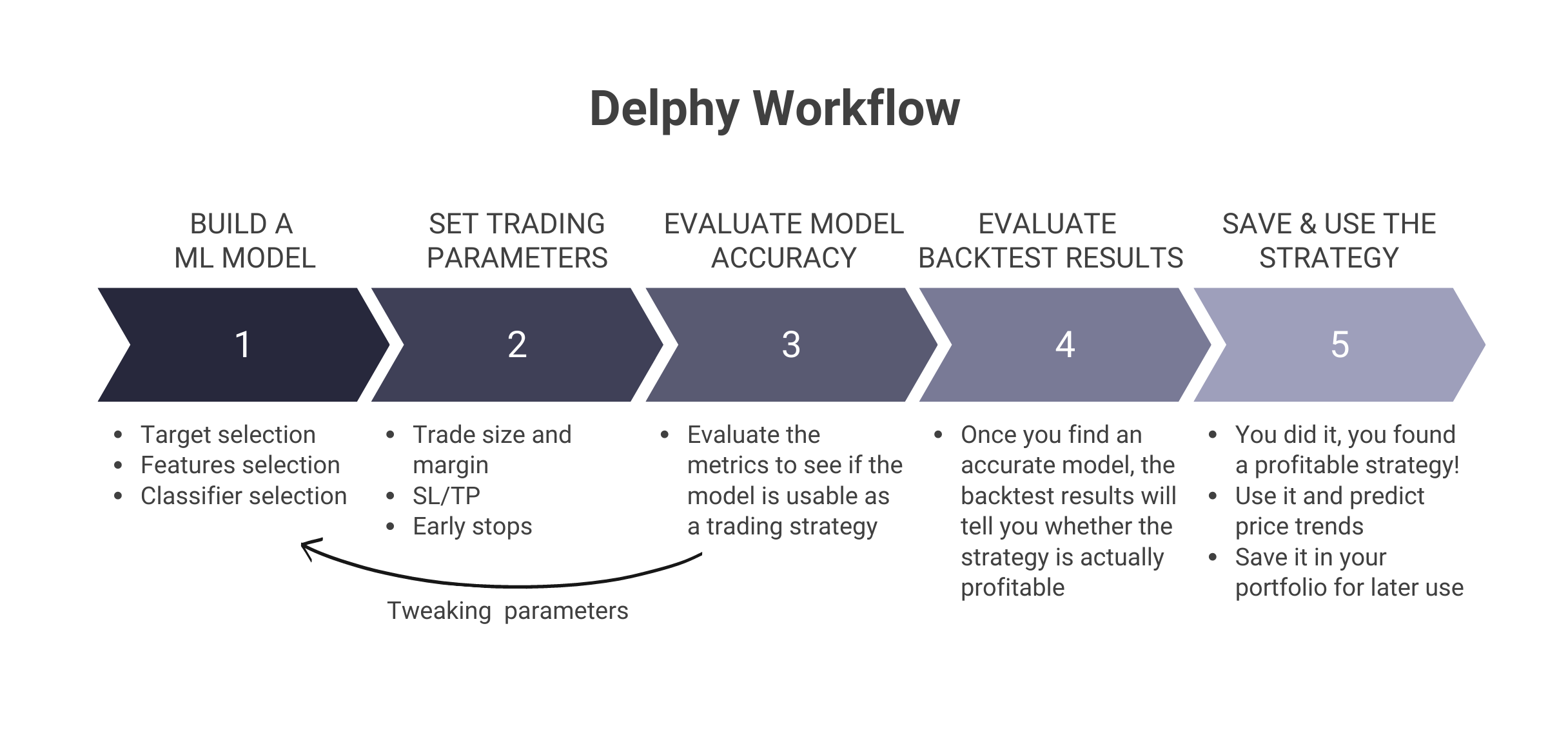
Delphy enables the creation of trading strategies by leveraging Machine Learning techniques. It allows you to train a model using historical data from various financial instruments such as stocks, forex, or crypto. You have the flexibility to select specific technical indicators that the model will consider during the training process. Once trained, Delphy evaluates the accuracy of the model by testing it on a separate dataset.
In addition to accuracy assessment, Delphy conducts a backtest to simulate the application of the strategy on the historical data, revealing how it would have performed if implemented during that time period. This evaluation helps you determine the viability and potential effectiveness of the strategy.
If you find the accuracy and backtest results satisfactory, you can proceed to utilize the strategy. Delphy stays updated with the most recent OHLCV (Open, High, Low, Close, Volume) data for the chosen financial instrument. It leverages the trained model to make predictions about the future price movement of the instrument for specific timeframes, such as 1, 2, 5, 15, or 30 days (based on your preference).
Using these predictions, you can make informed trading decisions. By analyzing the projected price trends, you can decide whether to initiate a Buy or Sell action, depending on your trading strategy.
Linear Models
Linear models in Machine Learning are a class of algorithms that establish a linear relationship between input features and output predictions.
Target Selection
To create a strategy, we must first define our target. We want to predict the price trend of a financial instrument, so we are going to select the symbol and how far into the future we want to make the prediction.
Instrument
Choose the financial instrument you want to analyze from:
- Stocks
- ETFs
- Cryptocurrencies
- Forex
- Indices
For example, if you want to analyze the stock of Apple, you can select the instrument "Stocks".
Symbol
Once the instrument is selected, you can indicate the symbol by typing it into the input field. By typing at least two characters, Delphy will suggest all symbols that begin with those.
Time Frame
After that, you can choose the time frame of the data you want to analyze. The time frame is the period during which data is considered for generating a single, aggregated data point.
The available time frames are:
- 1 minute
- 5 minutes
- 15 minutes
- 30 minutes
- 1 hour
- 4 hours
- 1 day
By choosing the time frame, you are setting the granularity of the financial data you are going to analyze.
How far?
Finally, you can choose how far into the future you want to make the prediction. The available options are:
- 1 Days
- 2 Days
- 5 Days
- 15 Days
- 30 Days
Features Selection
For feature selection, 4 different indicators can be chosen. See the section Technical Indicators for more information about the indicators.
Classifier Selection
As Linear Models, Delphy supports Linear Regression, Support Vector Machines (SVM), and K-nearest neighbors, which are popular linear models offering simplicity, efficiency, and adaptability in various trading scenarios.
In the table below, each selectable option is explained in detail.
Options:
| # | Classifier Name | Hyperparameters | Values |
|---|---|---|---|
| 1 | Logistic Regression A statistical method used for binary classification tasks, Logistic Regression estimates the probability of an outcome by fitting data to a logistic function. It is particularly useful when predicting binary events, such as stock prices going up or down. |
||
| Solver The optimization algorithm used to find the best-fitting parameters for the model. |
Large Linear Classification A highly efficient solver that utilizes a coordinate gradient descent algorithm. It is well-suited for high-dimensional and large-scale linear classification problems, but it may not perform well on datasets with a large number of samples. |
||
| Limited-memory Broyden-Fletcher-Goldfarb-Shanno A quasi-Newton optimization method that approximates the Hessian matrix using limited memory. It is well-suited for high-dimensional problems, as it is memory-efficient and converges faster than first-order methods. |
|||
| Newton-Conjugate Gradient An optimization algorithm that combines the benefits of both the Newton-Raphson and Conjugate Gradient methods. It is a second-order optimization technique that can handle large-scale problems efficiently, but it requires the computation of the Hessian matrix, which could be computationally expensive. |
|||
| Stochastic Average Gradient A variant of stochastic gradient descent that uses a random sample of previous gradient values to achieve faster convergence. It is suitable for large-scale datasets and converges faster than 'liblinear' when the number of samples is large. |
|||
| Stochastic Average Gradient descent with Acceleration An extension of the 'sag' method, providing improved convergence properties. It can handle non-smooth (L1) penalties, making it suitable for high-dimensional datasets and sparse logistic regression problems. |
|||
| C It controls the trade-off between achieving a low training error and maintaining a low model complexity. A smaller value of C creates a wider margin, allowing some misclassifications, while a larger value seeks to minimize misclassifications at the cost of a narrower margin. |
0.5 |
||
| 1 |
|||
| 2 | Support Vector Machine A supervised learning algorithm for classification and regression tasks, SVM aims to find the optimal hyperplane that best separates data points into different classes. This model is especially useful for handling complex, high-dimensional data. |
||
| Kernel It transforms input data into a higher-dimensional space to enable linear separation of classes when they are not linearly separable in the original space. |
Radial basis function (RBF) Also known as the Gaussian kernel, the RBF kernel maps input data to an infinite-dimensional space, making it a popular choice for handling non-linearly separable data. |
||
| Polynomial Kernel This kernel introduces a polynomial decision boundary in the input space. |
|||
| Sigmoid Kernel This kernel is inspired by the sigmoid activation function used in neural networks and can create non-linear decision boundaries. |
|||
| Decision Function Shape In the context of multi-class classification, it refers to the strategy used to extend binary classification methods, such as SVM, to handle multiple classes. |
One-vs-Rest This strategy involves training a separate binary classifier for each class, considering one class as the positive class and all other classes combined as the negative class. For a problem with 'n' classes, 'n' binary classifiers are trained. When making predictions, each classifier provides a score or probability for its respective class, and the class with the highest score or probability is chosen as the final prediction. The decision boundaries are created by combining the decision boundaries of individual classifiers. |
||
| One-vs-One In this strategy, a binary classifier is trained for every pair of classes, resulting in n(n-1)/2 classifiers for a problem with 'n' classes. Each classifier is trained to distinguish between its specific pair of classes, ignoring the data from other classes. During prediction, each classifier votes for its preferred class, and the class with the most votes is chosen as the final prediction. The decision boundaries in the input space are more complex, as they result from combining the decision boundaries of all pairwise classifiers. |
|||
| 3 | K-Nearest Neighbors A non-parametric, instance-based learning method used for classification and regression tasks. KNN works by finding the K nearest data points in the training set to a query point and making predictions based on the majority vote or the average of the neighbors' values. | ||
| No. of Neighbors |
2...8 |
Trading Strategy Parameters
To create a strategy, we must first define our target. We want to predict the price trend of a financial instrument, so we are going to select the symbol and how far into the future we want to make the prediction.
Cash
The initial cash to start with.
Trade Size
The size of the trade is calculated as a percentage of current available liquidity. Each time an order is placed (long or short) it will be by the indicated percentage. For example, if Trade size is 25% and the liquidity at that time is $1000, the order will be $250.
Leverage
Leverage in trading is using borrowed capital to amplify potential returns on investments. Option available for Forex and Crypto.
Commission
The commission is calculated as a percentage of the value of the trade.
Stop-Loss
The stop-loss value is calculated as a percentage of the price at the time the order is executed.
Take-Profit
The take-profit vale is calculated as a percentage of the price at the time the order is executed.
Early Stops
Select this option if you want to set aggressive stop-loss on trades that have been open for more than N days.
Accuracy Metrics
Accuracy metrics like AUC-ROC, MCC, Precision, and Recall are crucial in machine learning as they provide quantifiable measures to evaluate, compare, and improve the performance of models, ensuring they make reliable predictions and minimizing errors in decision-making processes.
MCC (Matthews Correlation Coefficient)
The MCC is a measure of the quality of binary classifications. It takes into account both overprediction and underprediction, and it returns a value between -1 and 1. An MCC of +1 represents a perfect prediction, 0 indicates no better than random prediction, and -1 demonstrates total disagreement between prediction and observation.
AUC-ROC (Area Under the Receiver Operating Characteristic Curve)
This metric measures the ability of a binary classifier to distinguish between positive and negative classes over a range of threshold settings. The ROC curve plots the True Positive Rate (sensitivity) against the False Positive Rate (1-specificity), and the AUC provides a single scalar value representing the expected performance of a classifier. An AUC of 1 indicates perfect classification, while an AUC of 0.5 suggests the classifier is no better than random guessing.
Precision (Positive Predictive Value)
Precision is the fraction of relevant instances among the retrieved instances. In other words, it is the number of true positives divided by the sum of true positives and false positives. It essentially asks the question, "Of all the instances the classifier labeled as positive, how many are actually positive?"
Recall (Sensitivity, True Positive Rate)
Recall is the fraction of total relevant instances that have been retrieved. In other words, it's the number of true positives divided by the sum of true positives and false negatives. It essentially asks the question, "Of all the actual positive instances, how many did the classifier correctly identify?"
Technical Indicators
Here we have a description of all the technical indicators in Delphy that are useful for training the ML model.
Support
If this documentation doesn't answer your questions, So, Please send us Email to support@delphy.ai
We are located in GMT +1 time zone and we answer all questions within 12-24 hours in weekdays. In some rare cases the waiting time can be to 48 hours. (except holiday seasons which might take longer).
Don’t forget to leave a Feedback here
Changelog
See what's new added, changed, fixed, improved or updated in the latest versions.
For Future Updates Follow Us @Reddit / @Facebook / @Twitter / @Instagram
Version 1.1 (10 May, 2023)
- Added Added Leverage for Forex and Crypto
- Fixed Some minor bugs for browser compatibility
- Fixed Some minor bugs for responsive
- Updated FontAwesome to Latest Version
- Updated Improvements in CSS and JS
Version 1.0 (30 April, 2023)
Initial Release